The stars library is a relatively new R framework for spatiotemporal arrays. In this demo, we will unpack a netcdf file to calculate the annual precipitation anomalies for southeastern Australia. This can also be effectively calculated using data frames, however my motivation here is to demonstrate how the stars array based workflow achieve this calculation faster and use far less memory.
library(tidyverse) # data wrangler
library(stars) # the *star* of this tutorial
library(lubridate) # date wrangler
library(googledrive) # download data
library(scico) # sci-viz color palettes
Here is a file with monthly averages for total precip, 2-m air temp, and 2-m dewpoint temperature that I got from the Copernicus Data Store for the ERA5-Land product.
fyi, the netcdf file is about 44 Mb.
Note that I am using stars::read_stars() instead of stars::read_ncdf
library(googledrive)
temp <- tempfile(fileext = ".nc")
dl <- googledrive::drive_download(
  as_id("1Fo5F--2tfWWZfhTKBOatfM-bDs2stjhB"), path = temp, overwrite = TRUE)
raw <- stars::read_stars(temp)
## d2m, t2m, tp,
Get summary of the raw file:
raw
## stars object with 3 dimensions and 3 attributes
## attribute(s), summary of first 1e+05 cells:
##     d2m [K]         t2m [K]          tp [m]
##  Min.   :271.7   Min.   :273.6   Min.   :0.000
##  1st Qu.:279.6   1st Qu.:285.4   1st Qu.:0.001
##  Median :281.2   Median :291.8   Median :0.001
##  Mean   :282.5   Mean   :291.9   Mean   :0.002
##  3rd Qu.:285.4   3rd Qu.:297.4   3rd Qu.:0.002
##  Max.   :295.0   Max.   :305.6   Max.   :0.016
##  NA's   :20998   NA's   :20998   NA's   :20998
## dimension(s):
##      from  to offset delta  refsys point                    values x/y
## x       1 131 140.95   0.1      NA    NA                      NULL [x]
## y       1 121 -26.95  -0.1      NA    NA                      NULL [y]
## time    1 483     NA    NA POSIXct    NA 1981-01-01,...,2021-03-01
Following the ERA5-Land documentation for ‘accumulation’ variables:
The accumulations in synoptic monthly means (stream=mnth) have units that include “variable_units per forecast_step hours”. So for accumulations in this stream:
The hydrological parameters are in units of “m of water equivalent per forecast_step hours” and so they should be multiplied by 1000 to convert to kgm-2 per forecast_step hours or mm per forecast_step hours.
So if I understood that correctly, we will multiply by 24 hours, and 1000 to get mm per month.
dp <- raw['tp']*(24*1000)
dp_y30 = aggregate(dp %>%
                   filter(time>=ymd("1981-01-01",tz='UTC')) %>%
                   filter(time<ymd("2011-01-01")),
                 by='year', sum)
dim(dp_y30)
## time    x    y
##   30  131  121
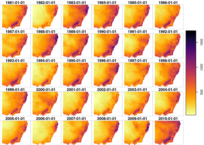
always plot! stars has nice and fast plotting functions which are great for sprinkling sanity checks throughout your analyses.
plot(dp_y30, breaks='equal', col=viridis::inferno(100,direction = -1))

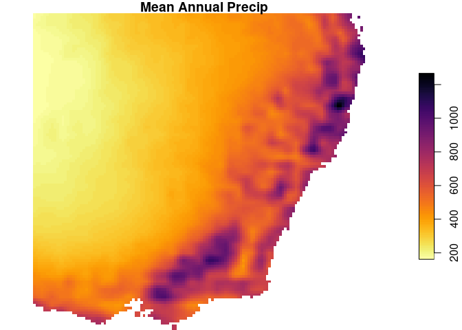
st_apply is our workhorse function here. Here we are just calculating the mean for each grid cell location ~ but we could do more complicated calculations such as rolling means, band-math, etc.
dp_map <- st_apply(dp_y30, MARGIN=c('x','y'), FUN=mean)
names(dp_map) <- 'MAP' # update the name
plot(dp_map, breaks='equal', col=viridis::inferno(100,direction = -1),
     main='Mean Annual Precip')

dp_y = aggregate(dp %>%
                   filter(time>=ymd("1981-01-01",tz='UTC')) %>%
                   filter(time<ymd("2021-01-01")),
                 by='year', sum)
dim(dp_y)
## time    x    y
##   40  131  121
So that is interesting. Any by interesting, I mean it’s a problem. The order of the dimensions is different from the input.
aperm is a standard array transposition function which stars can use to realign our aggregated stars object.
dp_y <- aperm(dp_y, perm = c(2,3,1))
dim(dp_y)
##    x    y time
##  131  121   40
Great, so now the array dimensions are consistent.
dp_anom <- dp_y-dp_map
## Warning in dim(e1) == dim(e2): longer object length is not a multiple of shorter
## object length
Note we get the warning because dp_y has a time dimension and dp_map does not. But stars can do the math so long as we maintain the standard order of dimensions: x,y,time
Update the name of the variable in dp_anom object:
names(dp_anom) <- 'precip_anom'
dp_anom
## stars object with 3 dimensions and 1 attribute
## attribute(s):
##   precip_anom
##  Min.   :-722.57
##  1st Qu.: -91.21
##  Median : -12.99
##  Mean   : -11.32
##  3rd Qu.:  65.29
##  Max.   : 666.14
##  NA's   :138280
## dimension(s):
##      from  to offset delta  refsys point                    values x/y
## x       1 131 140.95   0.1      NA    NA                      NULL [x]
## y       1 121 -26.95  -0.1      NA    NA                      NULL [y]
## time    1  40     NA    NA POSIXct    NA 1981-01-01,...,2020-01-01
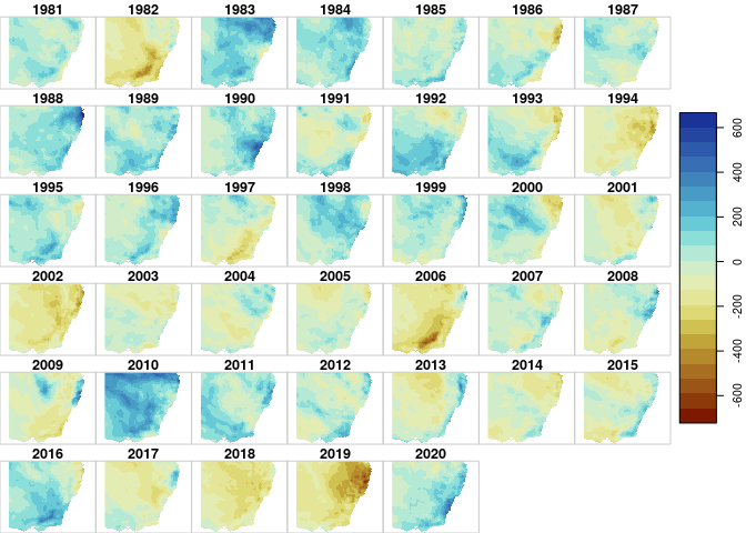
The time dimension is currently a POSIXct. This could be confused as the first date of each year, so let’s update them as a numeric corresponding to the calendar year.
dp_anom <- dp_anom %>%
  st_set_dimensions(., which = 3, values=1981:2020, names = 'year')
plot(dp_anom,
     join_zlim = T,
     breaks = 'equal',
     col=scico::scico(n=21, palette='roma'))

Ok, there are (at least) a couple of things here to nitpick. Should I have calculated the anomaly by some sort of hydraulic year instead of calendar year? Yes, probably. It is entirely possible to do this with stars, but I wanted to keep this example short and simple. Should I have retained the units from the original netcdf? Maybe, but I still drop them out of habit because I haven’t worked out how to (1) update them along the workflow, and (2) prevent them from breaking random functions. Maybe someday…
sessionInfo()
## R version 4.0.3 (2020-10-10)
## Platform: x86_64-pc-linux-gnu (64-bit)
## Running under: Pop!_OS 20.04 LTS
##
## Matrix products: default
## BLAS:   /usr/lib/x86_64-linux-gnu/openblas-pthread/libblas.so.3
## LAPACK: /usr/lib/x86_64-linux-gnu/openblas-pthread/liblapack.so.3
##
## locale:
##  [1] LC_CTYPE=en_US.UTF-8       LC_NUMERIC=C
##  [3] LC_TIME=en_US.UTF-8        LC_COLLATE=en_US.UTF-8
##  [5] LC_MONETARY=en_US.UTF-8    LC_MESSAGES=en_US.UTF-8
##  [7] LC_PAPER=en_US.UTF-8       LC_NAME=C
##  [9] LC_ADDRESS=C               LC_TELEPHONE=C
## [11] LC_MEASUREMENT=en_US.UTF-8 LC_IDENTIFICATION=C
##
## attached base packages:
## [1] stats     graphics  grDevices utils     datasets  methods   base
##
## other attached packages:
##  [1] scico_1.2.0       googledrive_1.0.1 lubridate_1.7.10  stars_0.5-2
##  [5] sf_0.9-8          abind_1.4-5       forcats_0.5.1     stringr_1.4.0
##  [9] dplyr_1.0.5       purrr_0.3.4       readr_1.4.0       tidyr_1.1.3
## [13] tibble_3.1.2      ggplot2_3.3.3     tidyverse_1.3.0
##
## loaded via a namespace (and not attached):
##  [1] Rcpp_1.0.6         class_7.3-17       assertthat_0.2.1   digest_0.6.27
##  [5] utf8_1.2.1         R6_2.5.0           cellranger_1.1.0   backports_1.2.1
##  [9] reprex_2.0.0       evaluate_0.14      e1071_1.7-6        highr_0.8
## [13] httr_1.4.2         pillar_1.6.1       rlang_0.4.11       readxl_1.3.1
## [17] rstudioapi_0.13    rmarkdown_2.7      munsell_0.5.0      proxy_0.4-25
## [21] broom_0.7.6        compiler_4.0.3     modelr_0.1.8       xfun_0.22
## [25] pkgconfig_2.0.3    htmltools_0.5.1.1  tidyselect_1.1.1   gridExtra_2.3
## [29] viridisLite_0.4.0  fansi_0.4.2        crayon_1.4.1       dbplyr_2.1.1
## [33] withr_2.4.1        grid_4.0.3         jsonlite_1.7.2     lwgeom_0.2-6
## [37] gtable_0.3.0       lifecycle_1.0.0    DBI_1.1.1          magrittr_2.0.1
## [41] units_0.7-1        scales_1.1.1       KernSmooth_2.23-17 cli_2.4.0
## [45] stringi_1.5.3      cubelyr_1.0.1      viridis_0.6.0      fs_1.5.0
## [49] xml2_1.3.2         ellipsis_0.3.2     generics_0.1.0     vctrs_0.3.8
## [53] tools_4.0.3        glue_1.4.2         hms_1.0.0          parallel_4.0.3
## [57] yaml_2.2.1         colorspace_2.0-0   classInt_0.4-3     rvest_1.0.0
## [61] knitr_1.31         haven_2.3.1